Prediction Overview

Updated on 07 Apr 2025
4 Minutes to read

Print
Share
Dark
Light

Article summary

Did you find this summary helpful?

Thank you for your feedback!

Overview

Predictive Modeling allows users to select a log or .CSV file and create a predictive model based on the variables.

Using Predictions

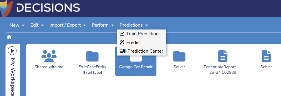
The Predictions menu can be found at the end of the Action menu. There are three available options a user can take: Train Prediction, Predict, and Prediction Center.

Train Prediction

Training Predictions takes available data and then creates a model from it. To train a Prediction, first select a log or .CSV. The Garage Car Repair data is an easy way to test this feature.

After selecting data and pressing Train Prediction, the following menu appears:

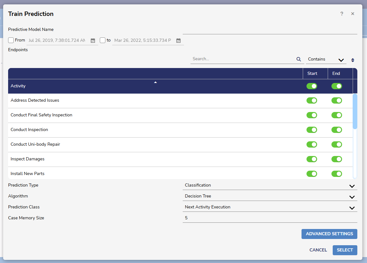
The Activity section contains all the attributes from the log or .CSV file.

Prediction Types

Type	Description
Classification	Predicts categories (Can be binary (1/0 or yes/no or Multiclass classification) Example: Binary Classification: Spam email detection – the Machine Learning model learns from previously labelled emails (spam/not spam) to identify new spam. Multiclass Classification: Predict drug class – the Machine Learning model learns from previously labelled patient data and drug prescribed to that patient (drugA, drugB, drugC) to identify which drug can be prescribed for the new patient data.
Regression	Predicts continuous numerical values. This determines relationships between the Prediction Class and one or more variables, in this case the attributes of the data. Example: House price prediction based on features like size, location, etc.

Type

Description

Classification

Predicts categories (Can be binary (1/0 or yes/no or Multiclass classification)

Example:

Binary Classification: Spam email detection – the Machine Learning model learns from previously labelled emails (spam/not spam) to identify new spam.

Multiclass Classification: Predict drug class – the Machine Learning model learns from previously labelled patient data and drug prescribed to that patient (drugA, drugB, drugC) to identify which drug can be prescribed for the new patient data.

Regression

Predicts continuous numerical values. This determines relationships between the Prediction Class and one or more variables, in this case the attributes of the data.

Example:

House price prediction based on features like size, location, etc.

Algorithm

Type	Description
Decision Tree	A decision tree is similar to a flowchart that makes decisions based on features. It can be used for both classification (DecisionTreeClassifier) and regression (DecisionTreeRegressor) tasks. Example: Predicting if a customer will buy a product based on their age and income.
Random Forest	Random Forest combines multiple decision trees to make more accurate predictions. Example: Predicting house prices based on various features like size, location, and number of rooms.
XGBoosted Trees	XGBoost is an advanced version of decision trees that builds trees sequentially, each correcting errors of the previous ones. Example: Predicting customer churn for a telecom company based on usage patterns and demographics.
Factorization Machines	Factorization Machines are a general-purpose supervised learning algorithm that can be used for both classification and regression tasks. This algorithm is good at capturing interactions between features. This is especially useful for recommendation systems. Example: Recommending movies to users based on their past ratings and movie features.
Kernel SVM	SVMs are supervised learning methods used for classification, regression and outliers' detection. SVM uses different types of kernels which are mathematical functions like Linear, Polynomial, Radial Basis Function and Sigmoid. Example: Classifying images of cats and dogs based on pixel values.
Linear Stochastic Gradient Descent	This is an optimization algorithm used in machine learning, particularly for linear models like linear regression and logistic regression. Compared to other optimization algorithms, LinearSGD can be faster for training linear models, especially when dealing with large datasets. This is because it avoids complex calculations needed for non-linear models. Linear Stochastic Gradient Descent is primarily suitable for linear models. It might not perform well with complex, non-linear models that require more sophisticated optimization techniques.
LibLinear	LibLinear is a library for large-scale linear classification, useful for text categorization or sentiment analysis. Example: Classifying news articles into categories like sports, politics, or technology.
LibSVM	This is a simple library for solving large-scale regularized linear classification and regression. It implements the sequential minimal optimization (SMO) algorithm for kernelized support vector machines (SVMs), supporting classification and regression.
Multinomial Naive Bayes	This algorithm is particularly useful for text classification tasks, assuming features are independent. Example: Classifying customer reviews as positive, negative, or neutral based on the words used.

Predict

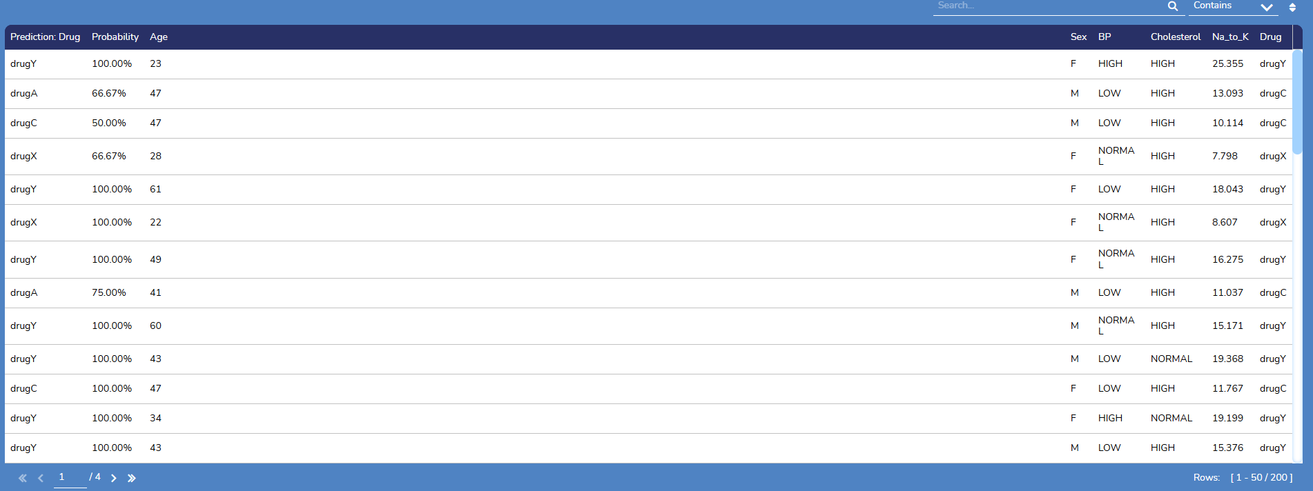
The Predict action allows the user to apply a prediction model against an imported log or .CSV file. As long as the file has the same characteristics as the model, it will provide a Probability column indicating how the data would perform.

Prediction Center

After a prediction model has been created, it can be found within the Prediction Center.

The name of the model. This is set when the model is created. It can be renamed at any time by right-clicking on the name.
The ID field is used to distinguish models from each other at the system level. When calling a model within Decisions, this ID number is critical.
The algorithm is determined at the time of creation. For more about the different types, see the section above.
Prediction class is the
Predictive models can have one of six different statuses.
1. Generating: This status will show up while the predictive model is still being trained.
2. Ready: This status will show up once the generation of the predictive model is completed.
3. Deployed: This status will show up for predictive models that are currently ready and deployed.
4. Ready (Unstable): This status will show up once the generation of the predictive model completed but the model is unstable. A model may be unstable when it is based on a classification algorithm, and it is not able to predict all possible target labels. Quality measures for unstable models are not available.
5. Deployed (Unstable): This status will show up for unstable predictive models that are currently ready and deployed.
6. Failed: This status will show up when the generation of the predictive model failed.
Actions

Icon	Name	Description
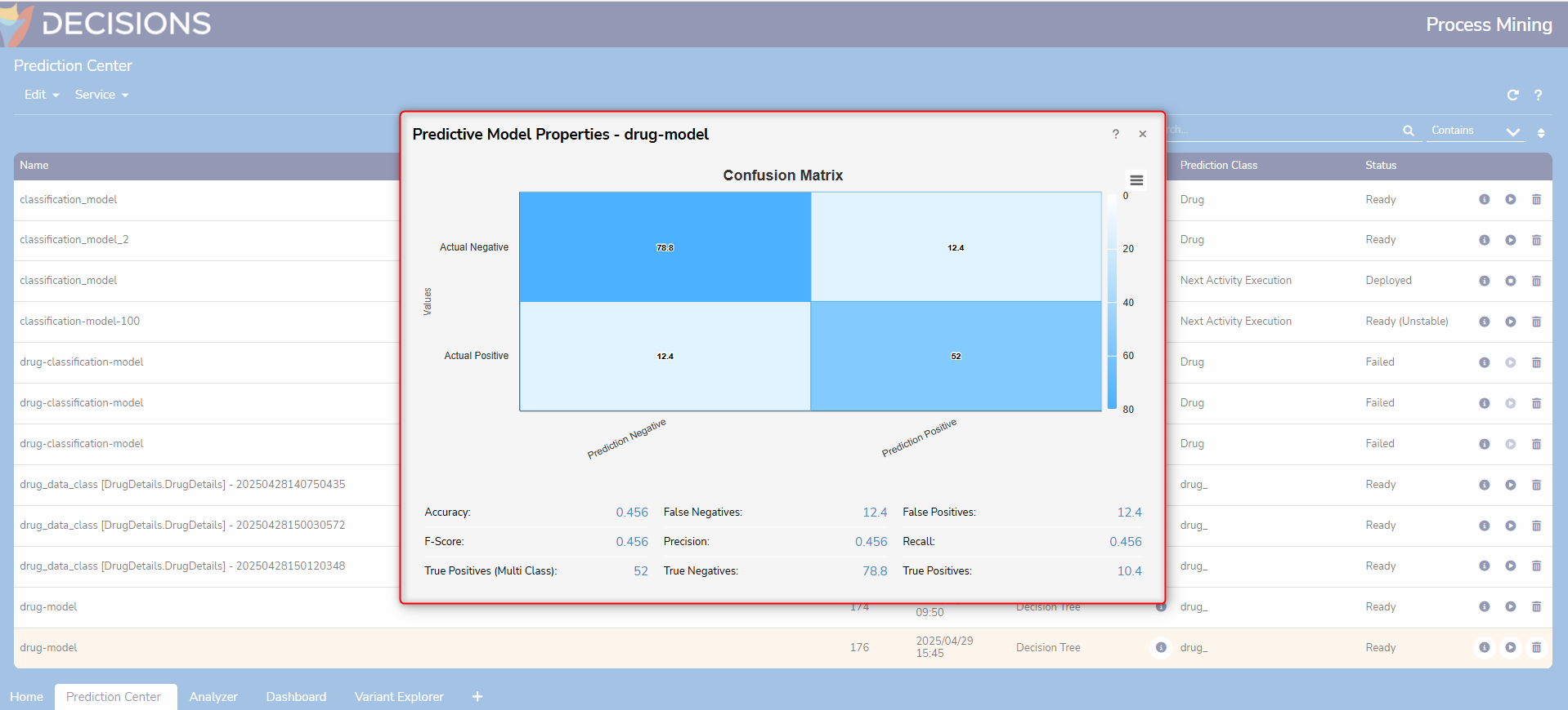
	Predictive Model Properties	This opens the Confusion Matrix screen, giving users insight into how the model will function.
	Ready	Changes the status of the model from Ready to Deployed.
	Delete	Deletes the highlighted model. There is no confirmation screen and this action is permanent. Be careful when using this action.

Was this article helpful?

Table of contents

Overview
Using Predictions
Predict
Prediction Center